reproducible-vignette
reproducible-vignette.RmdThis is a small, quick-running example showing how to use the SNPfiltR package to filter a next-generation sequencing (NGS) single nucleotide polymorphism (SNP) dataset. This vignette uses the small example dataset distributed with the package (20 samples, and 500 SNPs). The entire vignette can be rendered in <60s, allowing rapid validation of the filtering pipeline shown here. Overall, this pipeline shows the power of SNPfiltR to facilitate the visualization, exploration, and interactive filtering of any SNP dataset. We start by reading in our vcf file as a vcfR object. Having the vcfR object stored in local memory allows for the rapid visualization and imposition of various filtering criteria, allowing users to make informed decisions and interactively explore parameter space. This vignette follows best-practices by implementing quality aware filters (i.e., filters based on genotype quality) first, and quality blind filters (e.g., distance-based thinning) last, in order to preserve as many high-quality genotypes as possible for downstream analyses.
library(SNPfiltR)
#> This is SNPfiltR v.1.0.1
#>
#> Detailed usage information is available at: devonderaad.github.io/SNPfiltR/
#>
#> If you use SNPfiltR in your published work, please cite the following papers:
#>
#> DeRaad, D.A. (2022), SNPfiltR: an R package for interactive and reproducible SNP filtering. Molecular Ecology Resources, 00, 1-15. http://doi.org/10.1111/1755-0998.13618
#>
#> Knaus, Brian J., and Niklaus J. Grunwald. 2017. VCFR: a package to manipulate and visualize variant call format data in R. Molecular Ecology Resources, 17.1:44-53. http://doi.org/10.1111/1755-0998.12549
library(vcfR)
#>
#>    *****       ***   vcfR   ***       *****
#>    This is vcfR 1.14.0
#>      browseVignettes('vcfR') # Documentation
#>      citation('vcfR') # Citation
#>    *****       *****      *****       *****
Optional Step 0:
Do quality control per sample before performing SNP calling. I have written an RMarkdown script that uses the R package fastqcr to generate a report visualizing the quality and quantity of sequencing for each sample, and recommending a subset of samples to be immediately dropped before parameter optimization (specifically useful for RADseq data). The only modification necessary for this script is the path to the folder containing the input .fastq.gz files and the path to your desired output folder. An example report generated using this script can be seen here. Because the fastq.gz files for your experiment may be large and handled remotely, an example bash script for executing this RMarkdown file as a job on a high performance computing cluster is available here.
Step 1: read in vcf file as ‘vcfR’ object
Because we are using the example dataset distributed with the package, we just load in the vcf and popmap using the data() function.
#load the example vcfR object
data(vcfR.example)

### check the metadata present in your vcf
vcfR.example
#> ***** Object of Class vcfR *****
#> 20 samples
#> 1 CHROMs
#> 500 variants
#> Object size: 0.7 Mb
#> 38.07 percent missing data
#> *****        *****         *****

vcfR.example@fix[1:10,1:8]
#>       CHROM        POS        ID           REF ALT QUAL FILTER
#>  [1,] "Pseudochr1" "25801497" "16579:67:+" "A" "G" NA   "PASS"
#>  [2,] "Pseudochr1" "25457396" "16292:5:-"  "A" "G" NA   "PASS"
#>  [3,] "Pseudochr1" "20817192" "12868:12:-" "C" "T" NA   "PASS"
#>  [4,] "Pseudochr1" "29813636" "19560:94:+" "T" "C" NA   "PASS"
#>  [5,] "Pseudochr1" "28229092" "18530:62:-" "A" "G" NA   "PASS"
#>  [6,] "Pseudochr1" "9354478"  "4669:39:+"  "C" "T" NA   "PASS"
#>  [7,] "Pseudochr1" "17764465" "10787:26:+" "C" "T" NA   "PASS"
#>  [8,] "Pseudochr1" "5349729"  "1884:88:-"  "A" "T" NA   "PASS"
#>  [9,] "Pseudochr1" "17438085" "10478:65:-" "T" "G" NA   "PASS"
#> [10,] "Pseudochr1" "30854925" "20439:79:+" "G" "T" NA   "PASS"
#>       INFO
#>  [1,] "NS=93;AF=0.059"
#>  [2,] "NS=54;AF=0.056"
#>  [3,] "NS=109;AF=0.037"
#>  [4,] "NS=63;AF=0.016"
#>  [5,] "NS=97;AF=0.433"
#>  [6,] "NS=17;AF=0.059"
#>  [7,] "NS=103;AF=0.330"
#>  [8,] "NS=9;AF=0.111"
#>  [9,] "NS=16;AF=0.469"
#> [10,] "NS=102;AF=0.010"

vcfR.example@gt[1:10,1:2]
#>       FORMAT           A_californica_333849
#>  [1,] "GT:DP:AD:GQ:GL" "0/0:44:44,0:40:-0.00,-14.55,-152.08"
#>  [2,] "GT:DP:AD:GQ:GL" NA
#>  [3,] "GT:DP:AD:GQ:GL" "0/0:347:347,0:40:-0.00,-105.46,-1205.89"
#>  [4,] "GT:DP:AD:GQ:GL" "1/1:3:0,3:16:-9.57,-1.17,-0.03"
#>  [5,] "GT:DP:AD:GQ:GL" "0/1:67:33,34:40:-78.52,0.00,-75.77"
#>  [6,] "GT:DP:AD:GQ:GL" NA
#>  [7,] "GT:DP:AD:GQ:GL" "0/0:331:331,0:40:0.00,-99.80,-1063.41"
#>  [8,] "GT:DP:AD:GQ:GL" NA
#>  [9,] "GT:DP:AD:GQ:GL" NA
#> [10,] "GT:DP:AD:GQ:GL" "0/0:35:35,0:40:-0.00,-12.08,-112.81"

#Load the example popmap file. It is a standard two column popmap, where the first column must be named 'id' and contain individual sample identifiers matching the sample identifiers in the vcf file, and the second column must be named 'pop', and contain a population assignment for each sample.
data(popmap)
popmap
#>                       id          pop
#> 1   A_californica_333849  californica
#> 2   A_californica_333854  californica
#> 3   A_californica_333855  californica
#> 4   A_californica_333857  californica
#> 5   A_californica_333860  californica
#> 6     A_insularis_334031    insularis
#> 7     A_insularis_334032    insularis
#> 8     A_insularis_334033    insularis
#> 9     A_insularis_334034    insularis
#> 10    A_insularis_334037    insularis
#> 11  A_woodhouseii_334133  woodhouseii
#> 12  A_woodhouseii_334134  woodhouseii
#> 13  A_woodhouseii_334142  woodhouseii
#> 14  A_woodhouseii_334148  woodhouseii
#> 15  A_woodhouseii_334153  woodhouseii
#> 16 A_coerulescens_396256 coerulescens
#> 17 A_coerulescens_396259 coerulescens
#> 18 A_coerulescens_396262 coerulescens
#> 19 A_coerulescens_396263 coerulescens
#> 20 A_coerulescens_396264 coerulescens
Step 2: quality filtering
We now implement quality filters that don’t involve missing data. This is because removing low data samples will alter percentage/quantile based missing data cutoffs, so we wait to implement those until after deciding on our final set of samples for downstream analysis
#generate exploratory visualizations of depth and genotype quality for all called genotypes
#hard_filter(vcfR=vcfR.example)

#hard filter to minimum depth of 5, and minimum genotype quality of 30
vcfR<-hard_filter(vcfR=vcfR.example, depth = 5, gq = 30)
#> 28.81% of genotypes fall below a read depth of 5 and were converted to NA
#> 3.81% of genotypes fall below a genotype quality of 30 and were converted to NA
Jon Puritz has an excellent filtering tutorial that is focused specifically on filtering RADseq data.From Puritz SNP filtering tutorial “Allele balance: a number between 0 and 1 representing the ratio of reads showing the reference allele to all reads, considering only reads from individuals called as heterozygous, we expect that the allele balance in our data (for real loci) should be close to 0.5”. Here we will implement an allele balance filter converting called heterozygous genotypes outside of the .25-.75 range to NA.
#execute allele balance filter
vcfR<-filter_allele_balance(vcfR)
#> 7.54% of het genotypes (0.71% of all genotypes) fall outside of 0.25 - 0.75 allele balance ratio and were converted to NA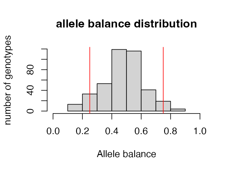
Here we will implement a max depth filter, as super high depth loci are likely multiple loci stuck together into a single paralogous locus, which we want to remove before making downstream inferences.
Note:
This filter is applied ‘per SNP’ rather than ‘per genotype’ otherwise we would simply be removing most of the genotypes from our deepest sequenced samples (because sequencing depth is so variable between samples). By filtering per SNP, we remove the SNPs with outlier depth values, which are most likely to be spuriously mapped/built paralagous loci.
#visualize and pick appropriate max depth cutoff
#max_depth(vcfR)
#not running here to save space on visualizations

#filter vcf by the max depth cutoff you chose
vcfR<-max_depth(vcfR, maxdepth = 100)
#> maxdepth cutoff is specified, filtered vcfR object will be returned
#> 17.6% of SNPs were above a mean depth of 100 and were removed from the vcf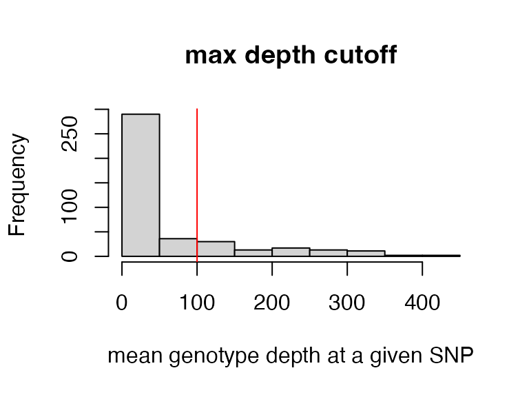
#check vcfR to see how many SNPs we have left
vcfR
#> ***** Object of Class vcfR *****
#> 20 samples
#> 2 CHROMs
#> 412 variants
#> Object size: 0.4 Mb
#> 67.65 percent missing data
#> *****        *****         *****
Step 3: set missing data per sample cutoff
Set arbitrary cutoff for missing data allowed per sample.
Determining which samples and SNPs to retain is always project specific, and is contingent on sampling, biology of the focal taxa, sequencing idiosyncrasies, etc. SNPfiltR contains functions designed to simply and easily generate exploratory visualizations that will allow you to make informed decisions about which samples and SNPs are of sufficient quality to retain for downstream analyses, but there is never a single correct option for these cutoffs. In my experience, the best thing to do is to look at your data, look at what effects some reasonable cutoffs would have on your data, and pick one that works for you. Then as you continue to analyze your data, make sure that your arbitrary filtering decisions are not driving the patterns you see, and iteratively update your filtering approach if you are concerned about the effects previous filtering choices are having on downstream results.
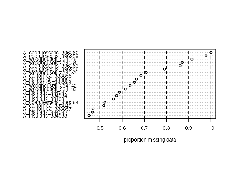
We are going to start by visualizing missing data per sample. After checking out the visualizations, we can make decision on which samples look like they will not be salvageable for downstream analysis, and remove them either by setting a data completeness cutoff in the function missing_by_sample(), or by name using base R syntax which works with vcfR objects which treat SNPs as rows and samples as columns (e.g., vcfR <- vcfR[,colnames(vcfR@gt) != “A_woodhouseii_24711”]).
Note:
If all of your samples are reasonably complete then you don’t need to drop any samples! Variable missing data by sample seems to be mostly an issue with RAD approaches for whatever reason.
#run function to visualize samples and return informative data.frame object
miss<-missing_by_sample(vcfR=vcfR)
#> No popmap provided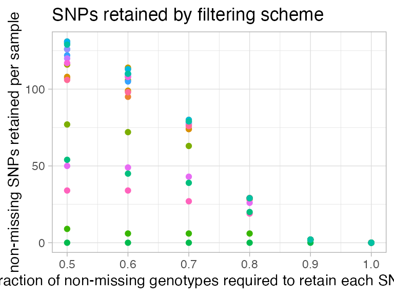
#run function to drop samples above the threshold we want from the vcf
#here I am setting a relatively lax cutoff
vcfR<-missing_by_sample(vcfR=vcfR, cutoff = .9)
#> 3 samples are above a 0.9 missing data cutoff, and were removed from VCF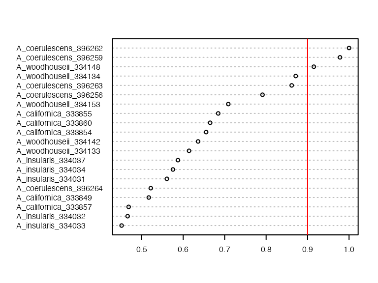
#remove invariant sites generated by sample trimming and genotype filtering
vcfR<-min_mac(vcfR, min.mac = 1)
#> 51.94% of SNPs fell below a minor allele count of 1 and were removed from the VCF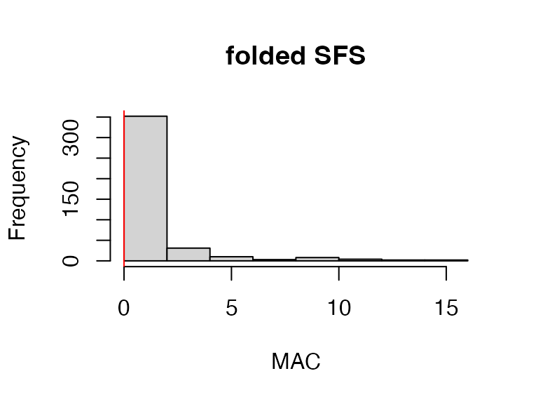
Step 4: set missing data per SNP cutoff
Set arbitrary cutoff for missing data allowed per SNP.
We can visualize the effect that typical missing data cutoffs will have on both the number of SNPs retained and the total missing data in our entire dataset.We want to choose a cutoff that minimizes the overall missing data in the dataset, while maximizing the total number of loci retained.
Note:
This filter interacts with the above filter, where we dropped low data samples. A good rule of thumb is that individual samples shouldn’t be above 50% missing data after applying a per-SNP missing data cutoff. So if we are retaining specific low data samples out of necessity or project design, we may have to set a more stringent per-SNP missing data cutoff, at the expense of the total number of SNPs retained for downstream analyses. We can again use the assess_missing_data_pca() function to determine whether all retained samples contain enough data at our chosen cutoff in order to be assigned accurately to their species group.
#visualize missing data by SNP and the effect of various cutoffs on the missingness of each sample
missing_by_snp(vcfR)
#> cutoff is not specified, exploratory visualizations will be generated
#> Picking joint bandwidth of 0.128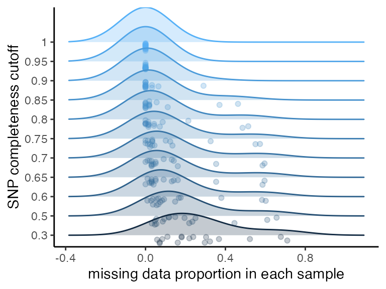
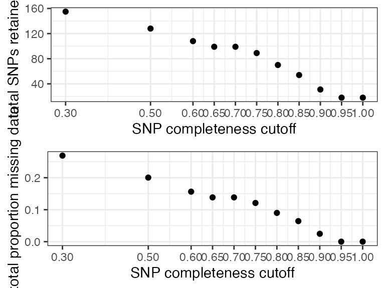
#> filt missingness snps.retained
#> 1 0.30 0.26907021 155
#> 2 0.50 0.20036765 128
#> 3 0.60 0.15631808 108
#> 4 0.65 0.13844326 99
#> 5 0.70 0.13844326 99
#> 6 0.75 0.12095175 89
#> 7 0.80 0.08991597 70
#> 8 0.85 0.06427015 54
#> 9 0.90 0.02466793 31
#> 10 0.95 0.00000000 18
#> 11 1.00 0.00000000 18We can see that there are still some outlier samples with a lot of missing data even at high missing data per SNP thresholds, which is concerning. We will want to check whether this excess missing data in some samples is affecting overall clustering patterns using the functions assess_missing_data_pca() and assess_missing_data_tsne().
#assess missing data effects on clustering
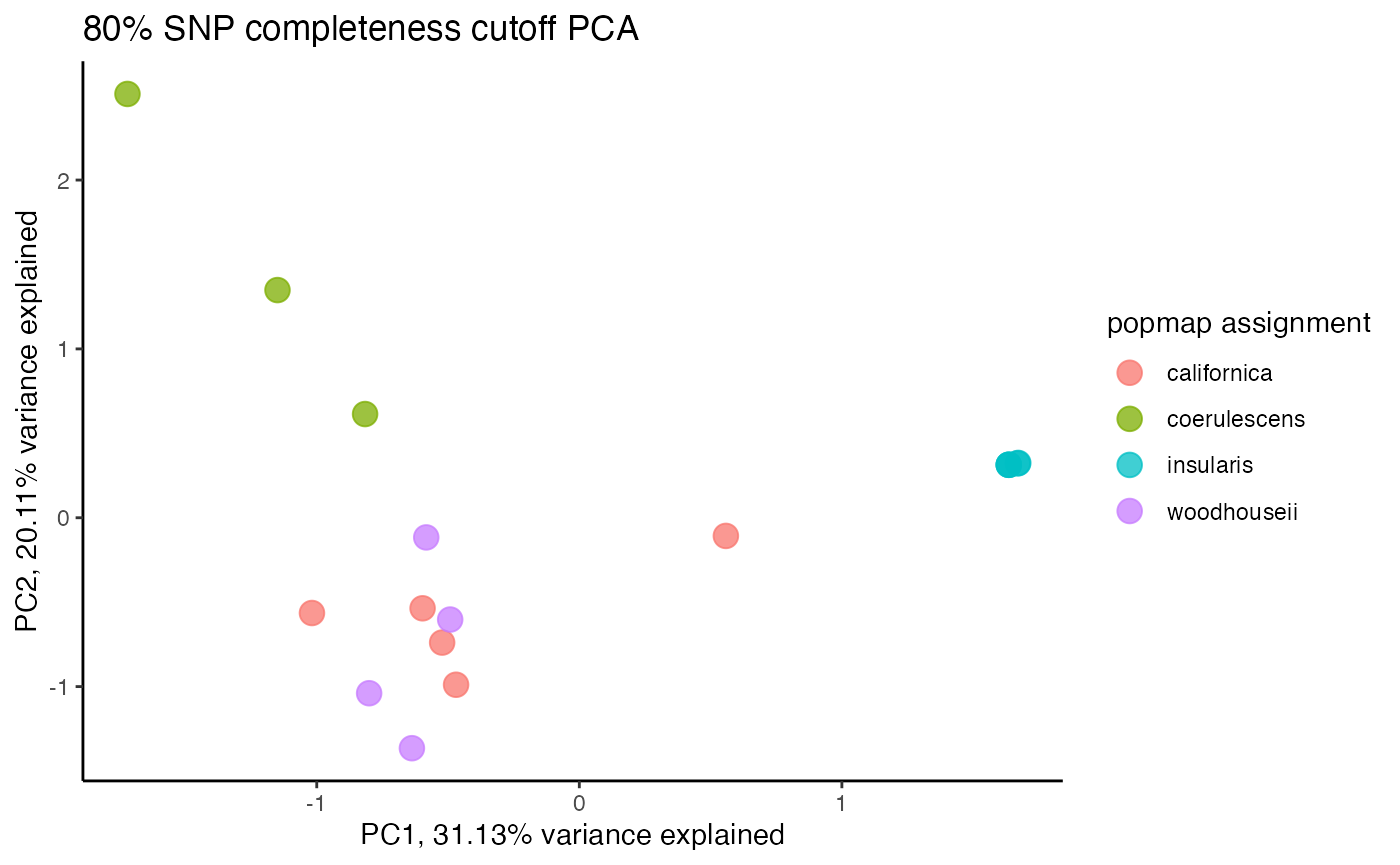
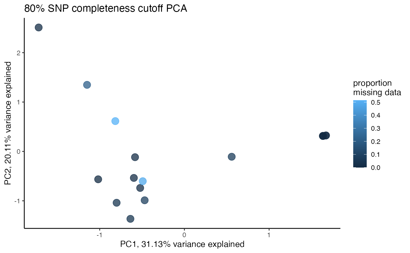
assess_missing_data_pca(vcfR = vcfR, popmap = popmap, thresholds = c(.8), clustering = FALSE)
#> cutoff is specified, filtered vcfR object will be returned
#> 64.65% of SNPs fell below a completeness cutoff of 0.8 and were removed from the VCF
#> Loading required namespace: adegenet
#> [[1]]
#> PC1 PC2 PC3 PC4
#> A_californica_333849 -0.5969622 -0.5362690 -0.595508158 0.73945078
#> A_californica_333854 -0.4693982 -0.9890245 -1.414869592 -1.37005171
#> A_californica_333855 0.5581980 -0.1075819 -0.257991833 0.14855832
#> A_californica_333857 -1.0182608 -0.5641853 -0.417897234 -0.28592615
#> A_californica_333860 -0.5224670 -0.7392822 -0.823298194 -0.01861634
#> A_insularis_334031 1.6356477 0.3136035 0.074824184 -0.03538247
#> A_insularis_334032 1.6717696 0.3245417 0.079829224 -0.03590089
#> A_insularis_334033 1.6695981 0.3219187 0.075663814 -0.03325062
#> A_insularis_334034 1.6356477 0.3136035 0.074824184 -0.03538247
#> A_insularis_334037 1.6356477 0.3136035 0.074824184 -0.03538247
#> A_woodhouseii_334133 -0.5830285 -0.1164268 -0.007498313 0.86818251
#> A_woodhouseii_334134 -0.4918528 -0.6028390 0.150783442 0.31303844
#> A_woodhouseii_334142 -0.8005397 -1.0392687 0.531437285 1.20318761
#> A_woodhouseii_334153 -0.6375918 -1.3648416 2.046665190 -1.05594446
#> A_coerulescens_396256 -1.1495480 1.3483650 0.060491990 0.14644120
#> A_coerulescens_396263 -0.8159388 0.6141574 0.121397651 -0.06714767
#> A_coerulescens_396264 -1.7209210 2.5099257 0.226322176 -0.44587363
#> PC5 PC6 pop missing
#> A_californica_333849 1.34940006 -0.217111195 californica 0.01428571
#> A_californica_333854 -0.31732671 -0.252236192 californica 0.08571429
#> A_californica_333855 0.79002290 -0.411529451 californica 0.07142857
#> A_californica_333857 -0.27279109 -0.675313989 californica 0.00000000
#> A_californica_333860 -0.29414891 1.230546314 californica 0.01428571
#> A_insularis_334031 -0.11699427 0.010904247 insularis 0.00000000
#> A_insularis_334032 -0.12438335 0.006458987 insularis 0.00000000
#> A_insularis_334033 -0.11649650 -0.001424441 insularis 0.01428571
#> A_insularis_334034 -0.11699427 0.010904247 insularis 0.00000000
#> A_insularis_334037 -0.11699427 0.010904247 insularis 0.00000000
#> A_woodhouseii_334133 0.22400118 0.462404897 woodhouseii 0.01428571
#> A_woodhouseii_334134 -0.05571374 0.543962142 woodhouseii 0.48571429
#> A_woodhouseii_334142 -1.18389174 -0.521504387 woodhouseii 0.04285714
#> A_woodhouseii_334153 0.44668940 0.174951057 woodhouseii 0.04285714
#> A_coerulescens_396256 0.01905756 0.014972030 coerulescens 0.21428571
#> A_coerulescens_396263 0.03051154 -0.599271664 coerulescens 0.51428571
#> A_coerulescens_396264 -0.14394778 0.212383154 coerulescens 0.01428571
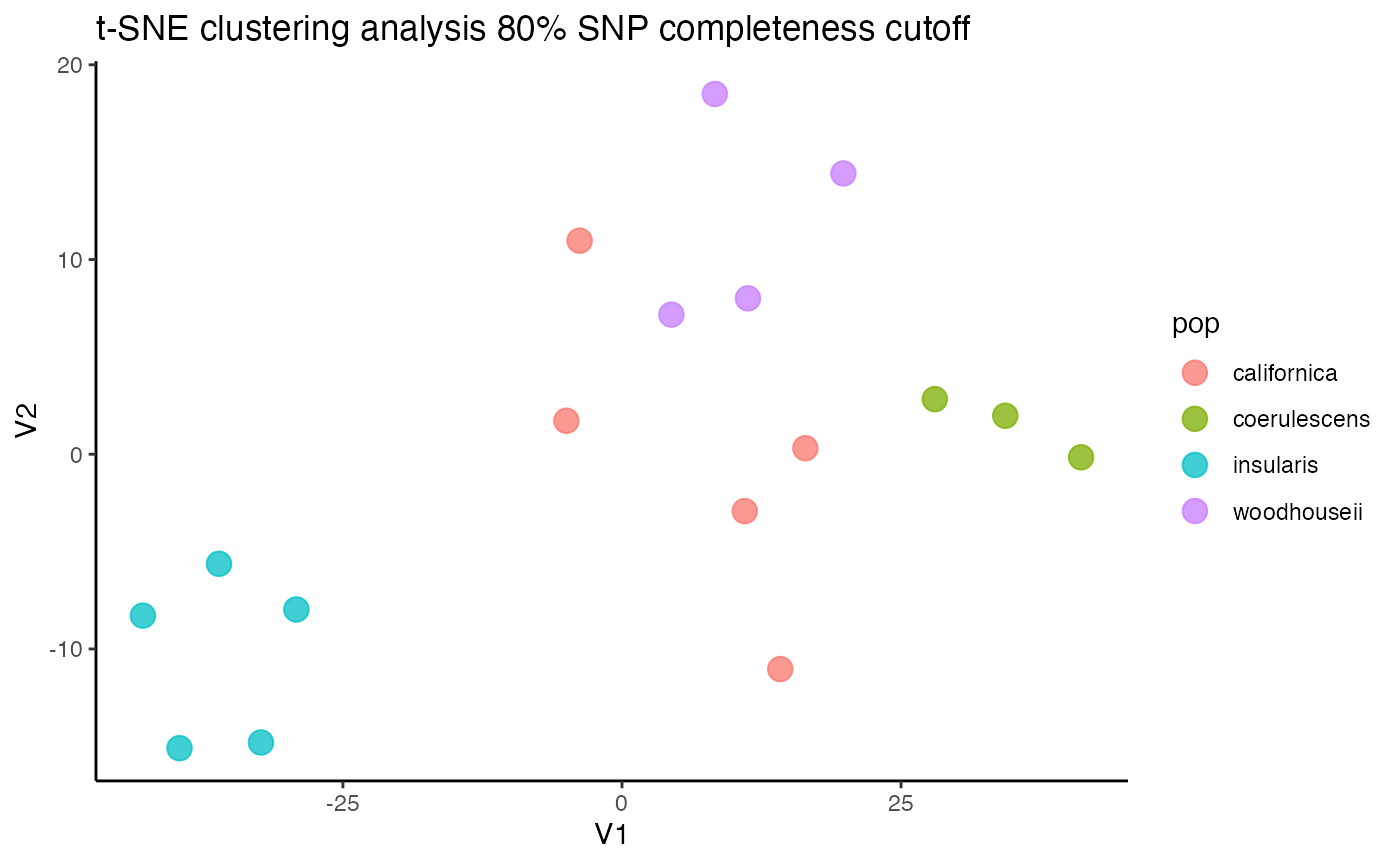
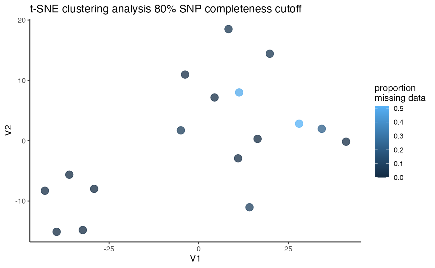
assess_missing_data_tsne(vcfR = vcfR, popmap = popmap, thresholds = c(.8), clustering = FALSE)
#> cutoff is specified, filtered vcfR object will be returned
#> 64.65% of SNPs fell below a completeness cutoff of 0.8 and were removed from the VCF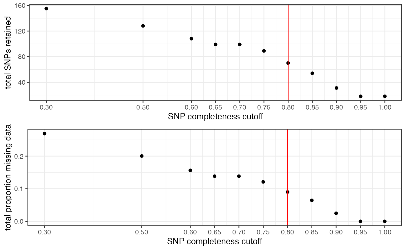
#> [[1]]
#> V1 V2 pop missing
#> 1 -3.796071 10.9680111 californica 0.01428571
#> 2 14.177537 -11.0327472 californica 0.08571429
#> 3 -4.983608 1.7200276 californica 0.07142857
#> 4 16.429284 0.3075205 californica 0.00000000
#> 5 10.998445 -2.9203174 californica 0.01428571
#> 6 -32.345592 -14.8051517 insularis 0.00000000
#> 7 -39.641833 -15.0977655 insularis 0.00000000
#> 8 -42.921031 -8.2889153 insularis 0.01428571
#> 9 -36.103795 -5.6274544 insularis 0.00000000
#> 10 -29.172878 -7.9731855 insularis 0.00000000
#> 11 4.424503 7.1709561 woodhouseii 0.01428571
#> 12 11.286257 8.0047602 woodhouseii 0.48571429
#> 13 8.318673 18.5033329 woodhouseii 0.04285714
#> 14 19.834320 14.4211641 woodhouseii 0.04285714
#> 15 34.338665 1.9770358 coerulescens 0.21428571
#> 16 28.027119 2.8296001 coerulescens 0.51428571
#> 17 41.130007 -0.1568713 coerulescens 0.01428571We can see that at an 80% per SNP completeness cutoff, samples with an excess of missing data are leaking toward the center (specifically coerulescens samples), indicating that they can’t be reliably clustered due to excess missing data.
We can go back and target specific samples with too much missing data even at high filtering thresholds for removal using the following code:
#show me the samples with the most missing data at an 80% completeness threshold
filt<-miss[miss$filt == .8,]
filt[order(filt$snps.retained),]
#> indiv filt snps.retained
#> 78 A_coerulescens_396262 0.8 0
#> 77 A_coerulescens_396259 0.8 6
#> 74 A_woodhouseii_334148 0.8 19
#> 79 A_coerulescens_396263 0.8 20
#> 72 A_woodhouseii_334134 0.8 26
#> 61 A_californica_333849 0.8 28
#> 62 A_californica_333854 0.8 29
#> 63 A_californica_333855 0.8 29
#> 64 A_californica_333857 0.8 29
#> 65 A_californica_333860 0.8 29
#> 66 A_insularis_334031 0.8 29
#> 67 A_insularis_334032 0.8 29
#> 68 A_insularis_334033 0.8 29
#> 69 A_insularis_334034 0.8 29
#> 70 A_insularis_334037 0.8 29
#> 71 A_woodhouseii_334133 0.8 29
#> 73 A_woodhouseii_334142 0.8 29
#> 75 A_woodhouseii_334153 0.8 29
#> 76 A_coerulescens_396256 0.8 29
#> 80 A_coerulescens_396264 0.8 29
#drop the three samples with an excess of missing data at an 80% SNP completeness threshold
vcfR<- vcfR[,colnames(vcfR@gt) != "A_coerulescens_396263" & colnames(vcfR@gt) != "A_woodhouseii_334134" & colnames(vcfR@gt) != "A_coerulescens_396256"]
#remove invariant SNPs
vcfR<-min_mac(vcfR, min.mac = 1)
#> 3.54% of SNPs fell below a minor allele count of 1 and were removed from the VCF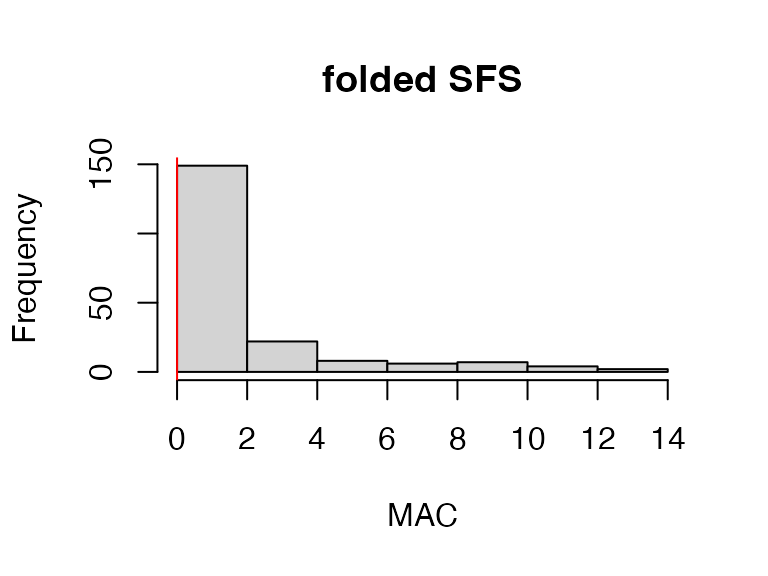
vcfR
#> ***** Object of Class vcfR *****
#> 14 samples
#> 1 CHROMs
#> 191 variants
#> Object size: 0.2 Mb
#> 31.71 percent missing data
#> ***** ***** *****
#update popmap by removing samples that have been filtered out
popmap<-popmap[popmap$id %in% colnames(vcfR@gt)[-1],]Re-visualize missing data by SNP and the effect of various cutoffs on the missingness of each sample and set a reasonable missing data cutoff.
#visualize missing data at various completeness thresholds
missing_by_snp(vcfR)
#> cutoff is not specified, exploratory visualizations will be generated
#> Picking joint bandwidth of 0.124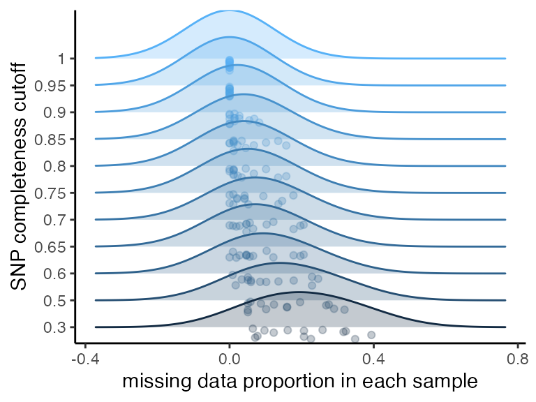
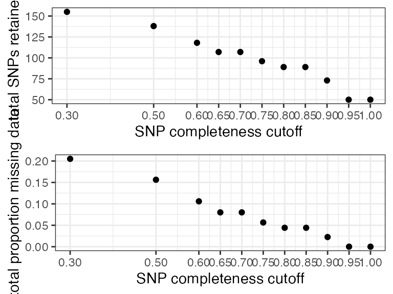
#>    filt missingness snps.retained
#> 1  0.30  0.20506912           155
#> 2  0.50  0.15631470           138
#> 3  0.60  0.10593220           118
#> 4  0.65  0.08010681           107
#> 5  0.70  0.08010681           107
#> 6  0.75  0.05654762            96
#> 7  0.80  0.04414125            89
#> 8  0.85  0.04414125            89
#> 9  0.90  0.02250489            73
#> 10 0.95  0.00000000            50
#> 11 1.00  0.00000000            50
#all samples look good at most thresholds, because of the small size of this dataset, I will choose a 60% completeness threshold in order to retain as many SNPs as possible

#filter vcfR
vcfR<-missing_by_snp(vcfR, cutoff = .6)
#> cutoff is specified, filtered vcfR object will be returned
#> 38.22% of SNPs fell below a completeness cutoff of 0.6 and were removed from the VCF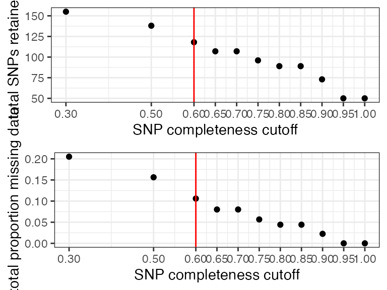
Step 5: quality unaware filters
We can now implement filters that are blind to genotype quality like a Minor Allele Count (MAC) threshold, and a distance-based filtering threshold, both of which may serve to increase the signal to noise ratio of our dataset in downstream analyses.
#remove singletons (loci with only a single variant allele which have no phylogenetic signal)
vcfR<-min_mac(vcfR = vcfR, min.mac = 2)
#> 38.14% of SNPs fell below a minor allele count of 2 and were removed from the VCF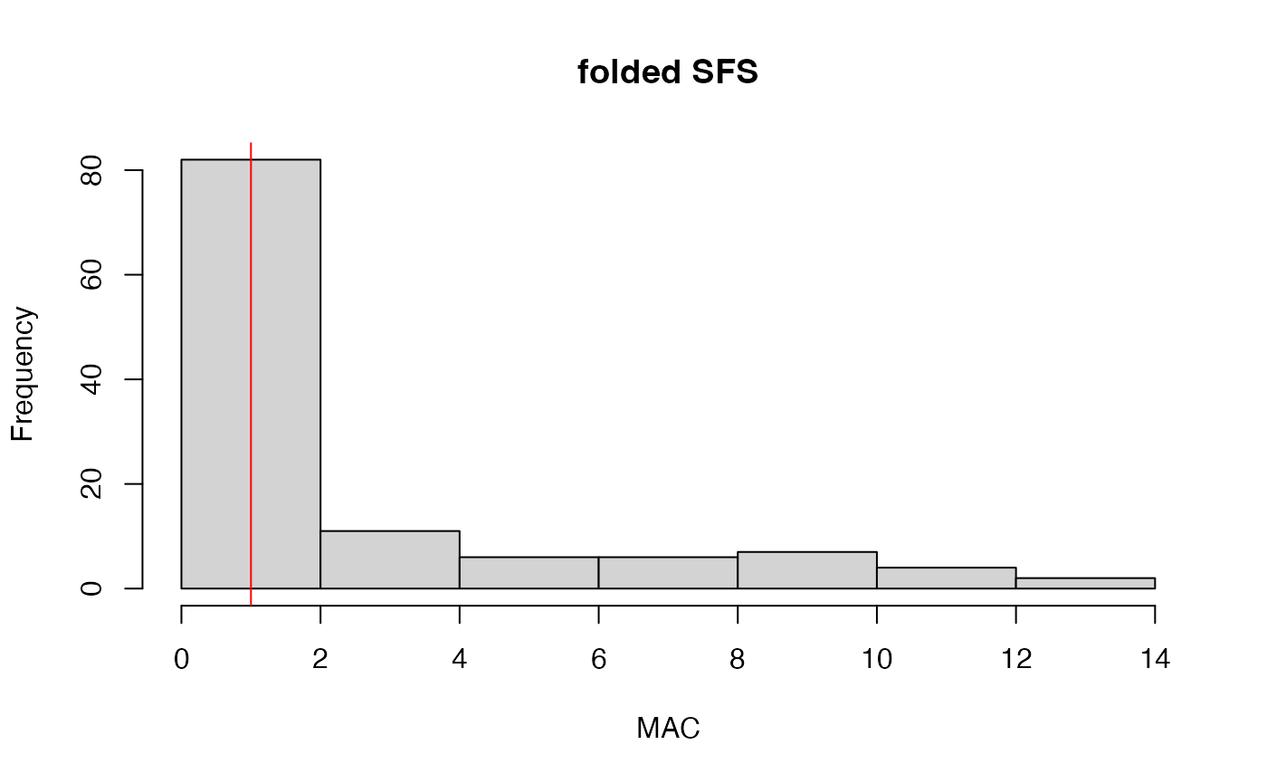
#linkage filter vcf to thin SNPs to one per 500bp
vcfR<-distance_thin(vcfR, min.distance = 500)
#>
  |
  |                                                                      |   0%
  |
  |======================================================================| 100%
#> 61 out of 73 input SNPs were not located within 500 base-pairs of another SNP and were retained despite filtering

#look at final stats for our filtered vcf file
vcfR
#> ***** Object of Class vcfR *****
#> 14 samples
#> 1 CHROMs
#> 61 variants
#> Object size: 0.1 Mb
#> 12.76 percent missing data
#> *****        *****         *****