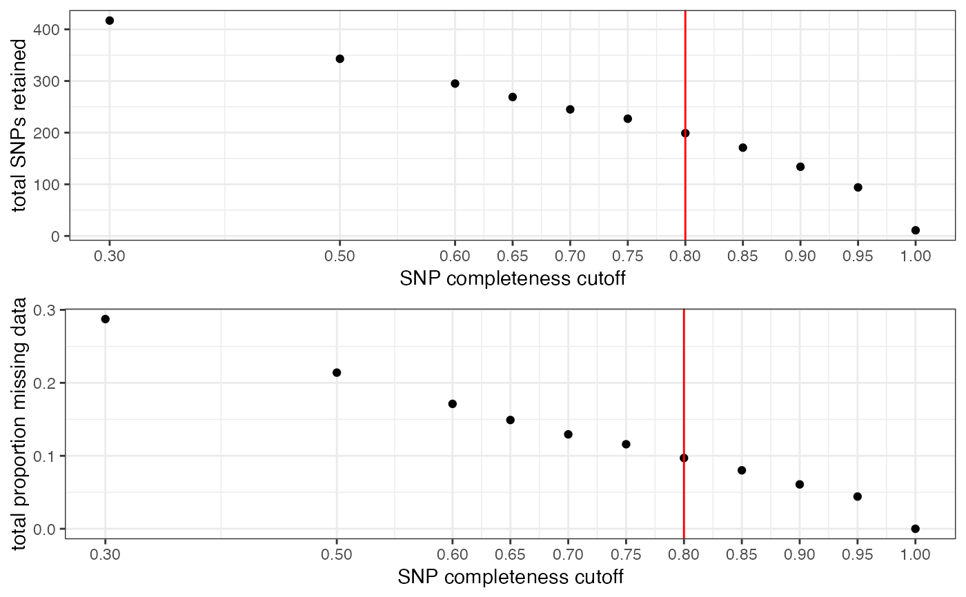
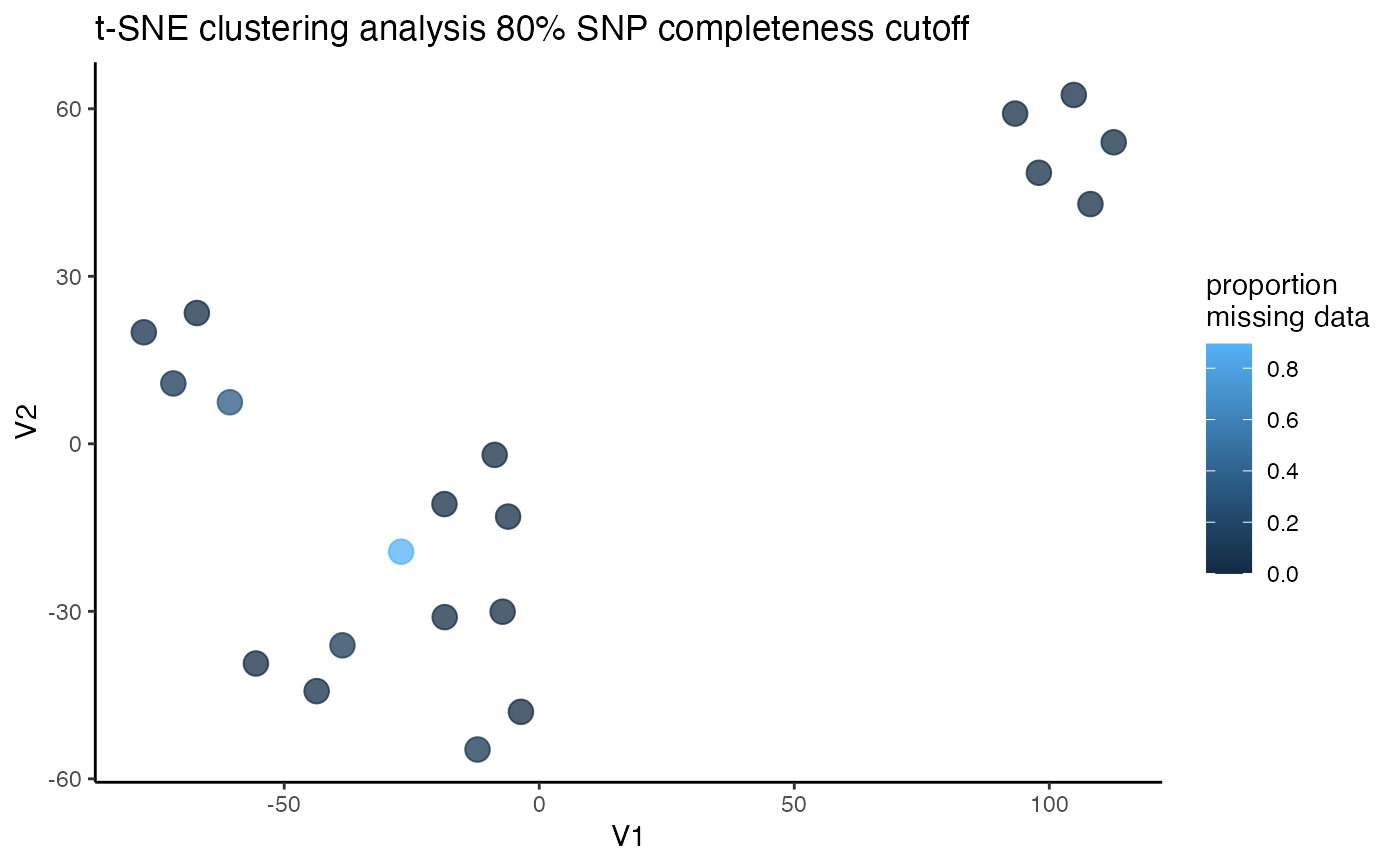
Vizualise how missing data thresholds affect sample clustering — assess_missing_data

This function can be run in two ways: 1) Without 'thresholds' specified. This will run t-SNE for the input vcf without filtering, and visualize the clustering of samples in two-dimensional space, coloring each sample according to a priori population assignment given in the popmap. 2) With 'thresholds' specified. This will filter your input vcf file to the specified missing data thresholds, and run a t-SNE clustering analysis for each filtering iteration. For each iteration, a 2D plot will be output showing clustering according to the specified popmap. This option is ideal for assessing the effects of missing data on clustering patterns.

assess_missing_data_tsne(
  vcfR,
  popmap = NULL,
  thresholds = NULL,
  perplexity = NULL,
  iterations = NULL,
  initial_dims = NULL,
  clustering = TRUE
)

Arguments

vcfR: a vcfR object
popmap: set of population assignments that will be used to color code the plots
thresholds: a vector specifying the missing data filtering thresholds to explore
perplexity: numerical value specifying the perplexity paramter during t-SNE (default: 5)
iterations: a numerical value specifying the number of iterations for t-SNE (default: 1000)
initial_dims: a numerical value specifying the number of initial_dimensions for t-SNE (default: 5)
clustering: use partitioning around medoids (PAM) to do unsupervised clustering on the output? (default = TRUE, max clusters = # of levels in popmap + 2)

Value

a series of plots showing the clustering of all samples in two-dimensional space

Examples

assess_missing_data_tsne(vcfR = SNPfiltR::vcfR.example,
popmap = SNPfiltR::popmap,
thresholds = .8)
#> cutoff is specified, filtered vcfR object will be returned
#> 65.8% of SNPs fell below a completeness cutoff of 0.8 and were removed from the VCF




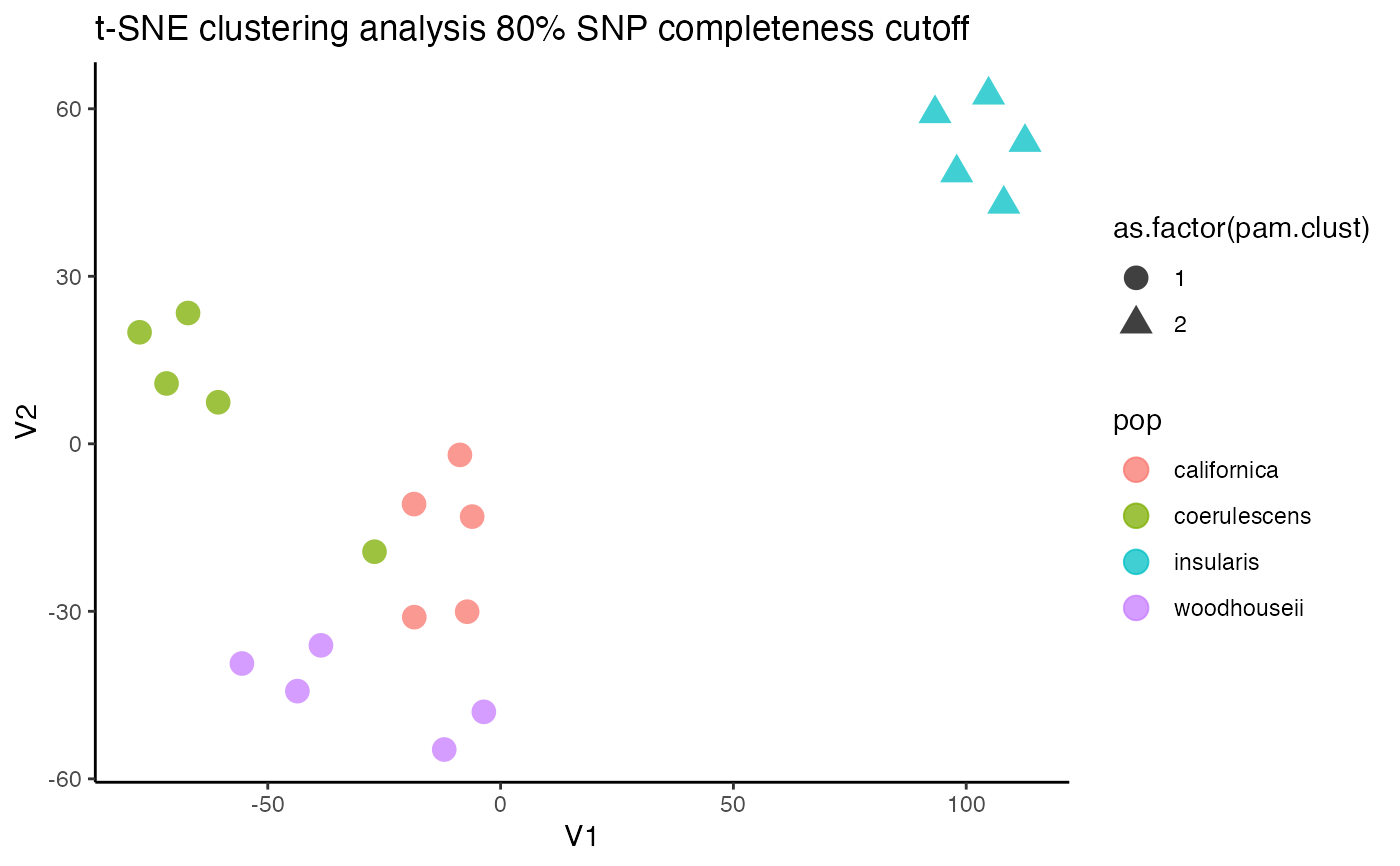
#> [[1]]
#>            V1         V2          pop pam.clust     missing
#> 1   -7.181015 -30.067725  californica         1 0.005847953
#> 2   -8.737704  -1.984322  californica         1 0.005847953
#> 3  -18.535683 -31.043675  californica         1 0.017543860
#> 4  -18.584513 -10.795087  californica         1 0.000000000
#> 5   -6.106049 -13.036955  californica         1 0.005847953
#> 6   97.957443  48.538775    insularis         2 0.005847953
#> 7  104.804006  62.472450    insularis         2 0.000000000
#> 8  108.065762  42.935323    insularis         2 0.005847953
#> 9  112.624444  54.000094    insularis         2 0.005847953
#> 10  93.297023  59.141590    insularis         2 0.000000000
#> 11  -3.595212 -48.000726  woodhouseii         1 0.000000000
#> 12 -12.102731 -54.750675  woodhouseii         1 0.076023392
#> 13 -55.552616 -39.344629  woodhouseii         1 0.000000000
#> 14 -38.583519 -36.090752  woodhouseii         1 0.116959064
#> 15 -43.640929 -44.292812  woodhouseii         1 0.011695906
#> 16 -77.530603  19.973745 coerulescens         1 0.029239766
#> 17 -60.653381   7.440146 coerulescens         1 0.327485380
#> 18 -27.077862 -19.325383 coerulescens         1 0.894736842
#> 19 -71.741261  10.808866 coerulescens         1 0.087719298
#> 20 -67.125596  23.421752 coerulescens         1 0.005847953
#>