This is a real example of using the RADstackshelpR package to facilitate parameter optimization on an empirical dataset. Bash code used to run the STACKS pipeline was executed via submit script on the KU high-performance computing cluster.

#load packages
library(RADstackshelpR)
library(gridExtra)

Step 1: Demultiplex each sample using ‘process_radtags’.

/home/path/to/stacks-2.41/process_radtags -p .  -o . -b plate.1.barcodes.txt -e ndeI -r -c -q

Step 2: Quality control - Once each sample has been demultiplexed into an individual file with the extension ‘.fastq.gz’, it is now possible to assess the quality of each sequenced sample. Samples which receive very little sequencing will not contain enough reads to assemble shared loci, and should be dropped right away, so that they do not bias the downstream optimization of assembly parameters. I have written an RMarkdown script that uses the R package fastqcr to generate a report visualizing the quality and quantity of sequencing for each sample, and recommending a subset of samples to be immediately dropped before parameter optimization. The only modification necessary for this script is the path to the folder containing the input .fastq.gz files and the path to your desired output folder. An example report generated using this script can be seen here.

Step 3: Now that we have run quality control, we have a reasonable set of samples for which to perform parameter optimization for de novo assembly. To begin, iterate over values of ‘m’ ranging from 3-7, while leaving all other parameters at default values.

###Bash code to execute this:

#!/bin/sh
#
#SBATCH --job-name=denovo.rad.hippo              # Job Name
#SBATCH --nodes=1             # nodes
#SBATCH --cpus-per-task=15               # CPU allocation per Task
#SBATCH --partition=bi            # Name of the Slurm partition used
#SBATCH --chdir=/home/d669d153/scratch/diadema.dinops   # Set working d$
#SBATCH --mem-per-cpu=1gb            # memory requested
#SBATCH --time=10000

files="908108_H_diadema_Gatokae
908150_H_dinops_Guadalcanal
908151_H_diadema_Guadalcanal
908152_H_diadema_Guadalcanal
908153a_H_dinops_Guadalcanal
908154_H_dinops_Guadalcanal
908155_H_dinops_Guadalcanal
908156_H_diadema_Guadalcanal
908208_H_diadema_Guadalcanal
KVO150_H_diadema_Isabel
KVO168_H_diadema_Isabel
KVO169_H_diadema_Isabel
KVO170_H_diadema_Isabel
KVO171_H_diadema_Isabel
KVO172_H_diadema_Isabel
KVO242_H_dinops_Isabel
KVO243_H_dinops_Isabel
KVO244_H_dinops_Isabel
KVO245_H_dinops_Isabel
KVO246_H_dinops_Isabel
KVO248_H_dinops_Isabel
THL1156_H_demissus_Makira
THL1172_H_dinops_Guadalcanal
THL1173_H_dinops_Guadalcanal
THL17193_H_diadema_Ngella
THL17194_H_diadema_Ngell
THL17195_H_diadema_Ngella
THL17197_H_diadema_Ngella
THL17198_H_diadema_Ngella
THL17199_H_diadema_Ngell
WD1705_H_diadema_E_New_Britain
WD2047_H_diadema_Simbu_Prov
WD2074_H_diadema_Gulf_Prov"

# Build loci de novo in each sample for the single-end reads only.
# -M — Maximum distance (in nucleotides) allowed between stacks (default 2).
# -m — Minimum depth of coverage required to create a stack (default 3).
#here, we will vary m from 3-7, and leave all other paramaters default

for i in {3..7}
do
#create a directory to hold this unique iteration:
mkdir stacks_m$i
#run ustacks with m equal to the current iteration (3-7) for each sample
id=1
for sample in $files
do
    /home/d669d153/work/stacks-2.41/ustacks -f ${sample}.fq.gz -o stacks_m$i -i $id -m $i -p 15
    let "id+=1"
done
## Run cstacks to compile stacks between samples. Popmap is a file in working directory called 'pipeline_popmap.txt'
/home/d669d153/work/stacks-2.41/cstacks -P stacks_m$i -M pipeline_popmap.txt -p 15
## Run sstacks. Match all samples supplied in the population map against the catalog.
/home/d669d153/work/stacks-2.41/sstacks -P stacks_m$i -M pipeline_popmap.txt -p 15
## Run tsv2bam to transpose the data so it is stored by locus, instead of by sample.
/home/d669d153/work/stacks-2.41/tsv2bam -P stacks_m$i -M pipeline_popmap.txt -t 15
## Run gstacks: build a paired-end contig from the metapopulation data (if paired-reads provided),
## align reads per sample, call variant sites in the population, genotypes in each individual.
/home/d669d153/work/stacks-2.41/gstacks -P stacks_m$i -M pipeline_popmap.txt -t 15
## Run populations completely unfiltered and output unfiltered vcf, for input to the RADstackshelpR package
/home/d669d153/work/stacks-2.41/populations -P stacks_m$i -M pipeline_popmap.txt --vcf -t 15
done

Note: The vcf file output by Stacks containing only variant site information for each sample will be called ‘populations.snps.vcf’, unless you renamed it yourself by setting the -o flag in populations. This is the vcf file that you want to use for input to RADstackshelpR functions.

Step 4: Visualize the output of these 5 runs and determine the optimal value for m.

#optimize_m function will generate summary stats on your 5 iterative runs
#input can be full path to each file or just the file name if your working directory contains the files
m.out<-optimize_m(m3="/Users/devder/Desktop/hipposideros/m_3.vcf",
           m4="/Users/devder/Desktop/hipposideros/m_4.vcf",
           m5="/Users/devder/Desktop/hipposideros/m_5.vcf",
           m6="/Users/devder/Desktop/hipposideros/m_6.vcf",
           m7="/Users/devder/Desktop/hipposideros/m_7.vcf")

#visualize the effect of varying m on the depth of each sample
vis_depth(output = m.out)
#> [1] "Visualize how different values of m affect average depth in each sample"
#> Picking joint bandwidth of 9.53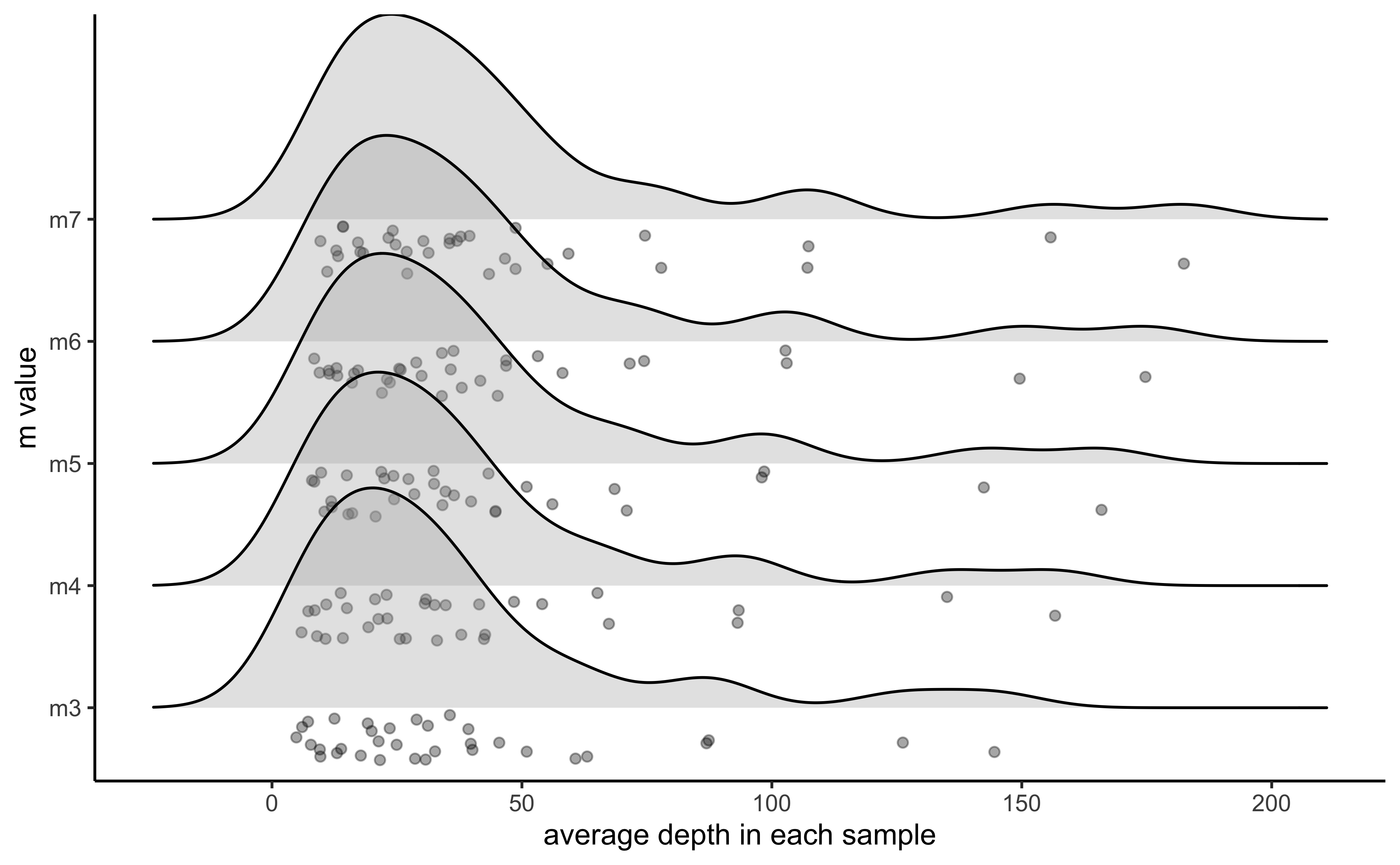

#visualize the effect of varying m on the number of SNPs retained
vis_snps(output = m.out, stacks_param = "m")
#> Visualize how different values of m affect number of SNPs retained.
#> Density plot shows the distribution of the number of SNPs retained in each sample,
#> while the asterisk denotes the total number of SNPs retained at an 80% completeness cutoff.
#> Picking joint bandwidth of 7190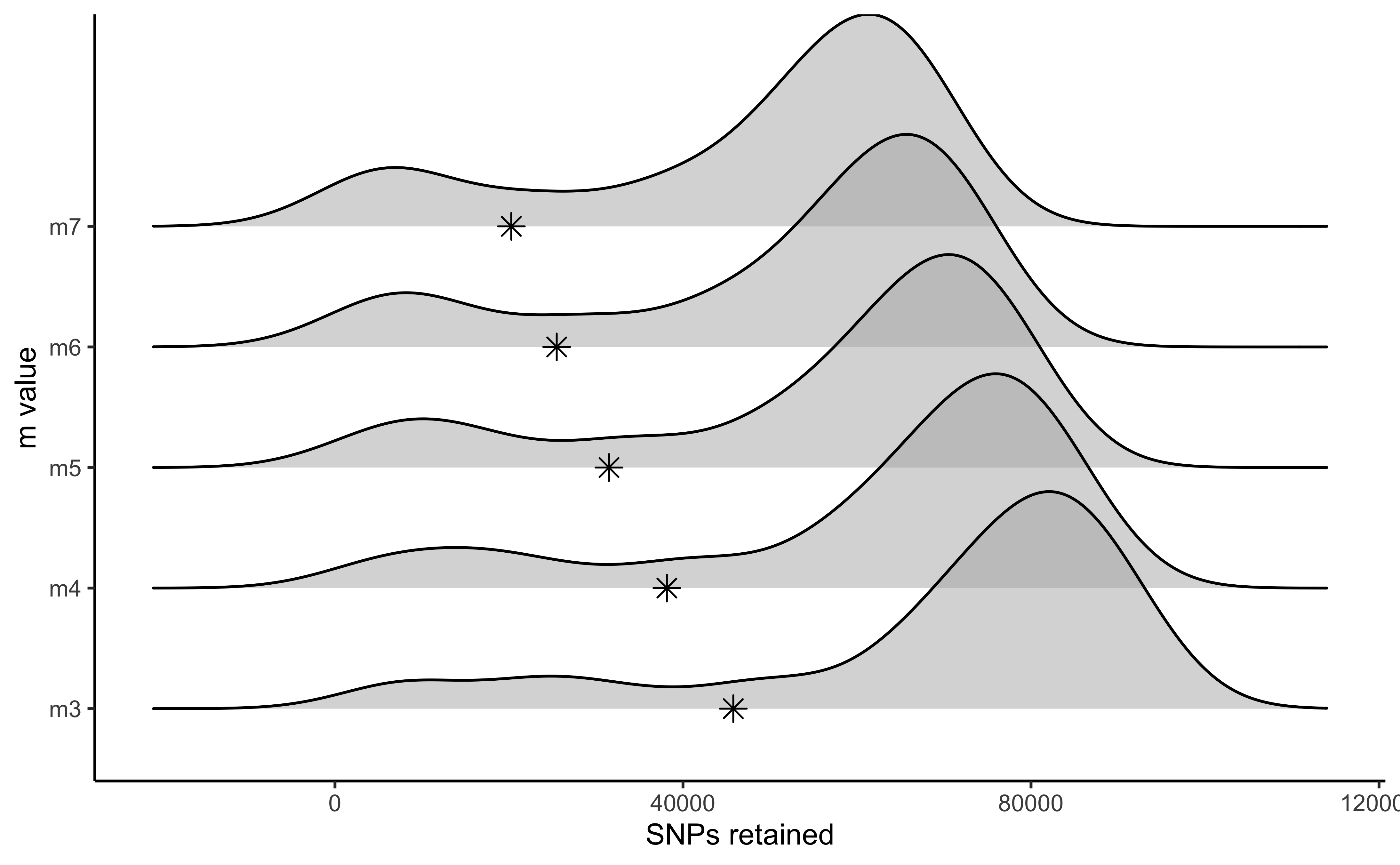


#visualize the effect of varying m on the number of loci retained
vis_loci(output = m.out, stacks_param = "m")
#> Visualize how different values of m affect number of polymorphic loci retained.
#> Density plot shows the distribution of the number of loci retained in each sample,
#> while the asterisk denotes the total number of loci retained at an 80% completeness cutoff. The optimal value is denoted by red color.
#> Picking joint bandwidth of 3420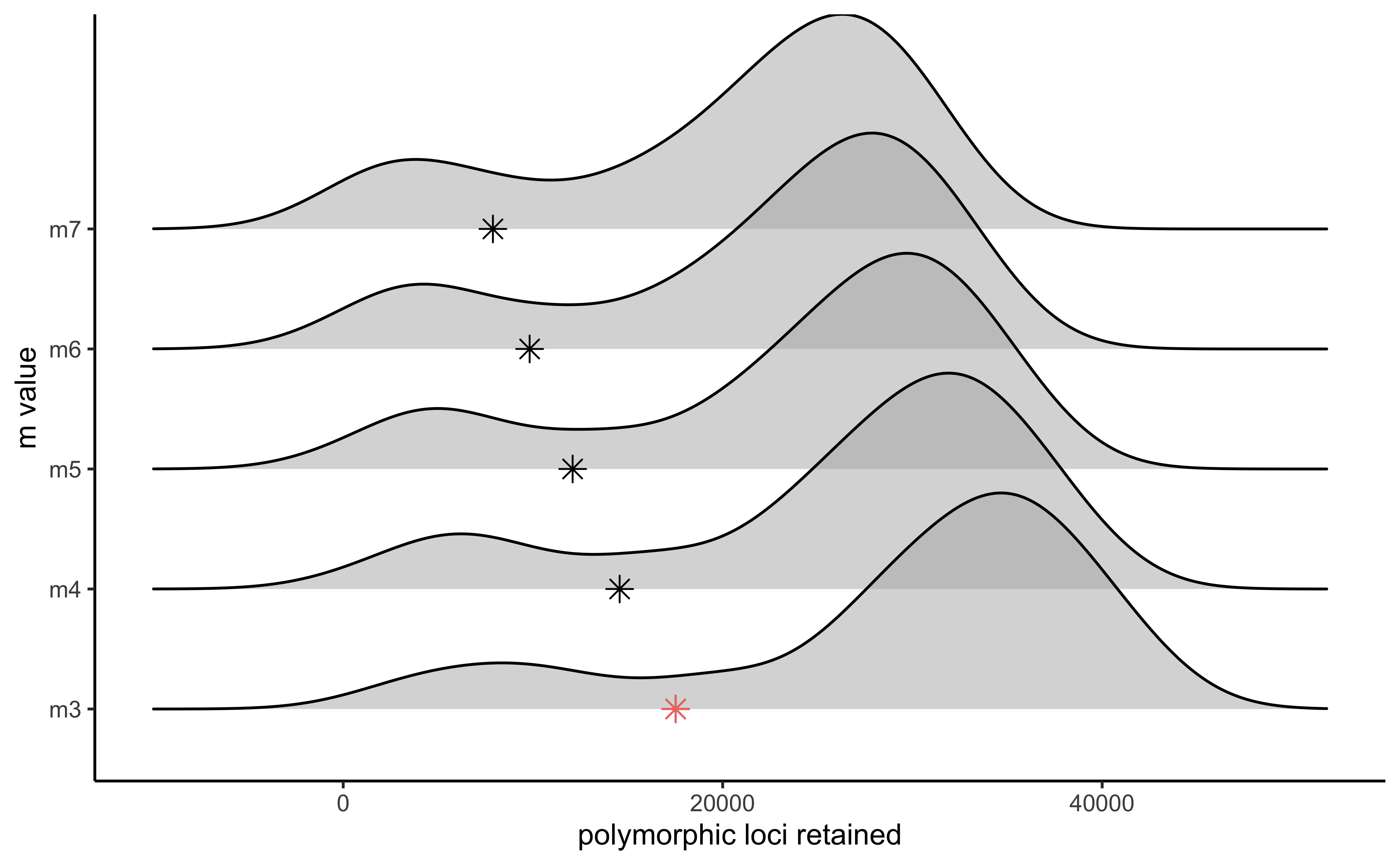


#3 is the optimal m value, and will be used next to optimize M

Step 5: Iterate over values of M ranging from 1-8, setting m to the optimal value (here 3).

This code follows the bash chunk above, utilizing the same variable $files

# -M — Maximum distance (in nucleotides) allowed between stacks (default 2).
# -m — Minimum depth of coverage required to create a stack (default 3).
#here, vary M from 1-8, and set m to the optimized value based on prior visualizations (here 3)
for i in {1..8}
do
#create a directory to hold this unique iteration:
mkdir stacks_bigM$i
#run ustacks with M equal to the current iteration (1-8) for each sample, and m set to the optimized value (here, m=3)
id=1
for sample in $files
do
    /home/d669d153/work/stacks-2.41/ustacks -f ${sample}.fq.gz -o stacks_bigM$i -i $id -m 3 -M $i -p 15
    let "id+=1"
done
/home/d669d153/work/stacks-2.41/cstacks -P stacks_bigM$i -M pipeline_popmap.txt -p 15
/home/d669d153/work/stacks-2.41/sstacks -P stacks_bigM$i -M pipeline_popmap.txt -p 15
/home/d669d153/work/stacks-2.41/tsv2bam -P stacks_bigM$i -M pipeline_popmap.txt -t 15
/home/d669d153/work/stacks-2.41/gstacks -P stacks_bigM$i -M pipeline_popmap.txt -t 15
/home/d669d153/work/stacks-2.41/populations -P stacks_bigM$i -M pipeline_popmap.txt --vcf -t 15
done

Step 6: Visualize the output of these 8 runs and determine the optimal value for M.

#optimize M
M.out<-optimize_bigM(M1="/Users/devder/Desktop/hipposideros/M1.vcf",
           M2="/Users/devder/Desktop/hipposideros/M2.vcf",
           M3="/Users/devder/Desktop/hipposideros/M3.vcf",
           M4="/Users/devder/Desktop/hipposideros/M4.vcf",
           M5="/Users/devder/Desktop/hipposideros/M5.vcf",
           M6="/Users/devder/Desktop/hipposideros/M6.vcf",
           M7="/Users/devder/Desktop/hipposideros/M7.vcf",
           M8="/Users/devder/Desktop/hipposideros/M8.vcf")

#visualize the effect of varying M on the number of SNPs retained
vis_snps(output = M.out, stacks_param = "M")
#> Visualize how different values of M affect number of SNPs retained.
#> Density plot shows the distribution of the number of SNPs retained in each sample,
#> while the asterisk denotes the total number of SNPs retained at an 80% completeness cutoff.
#> Picking joint bandwidth of 6090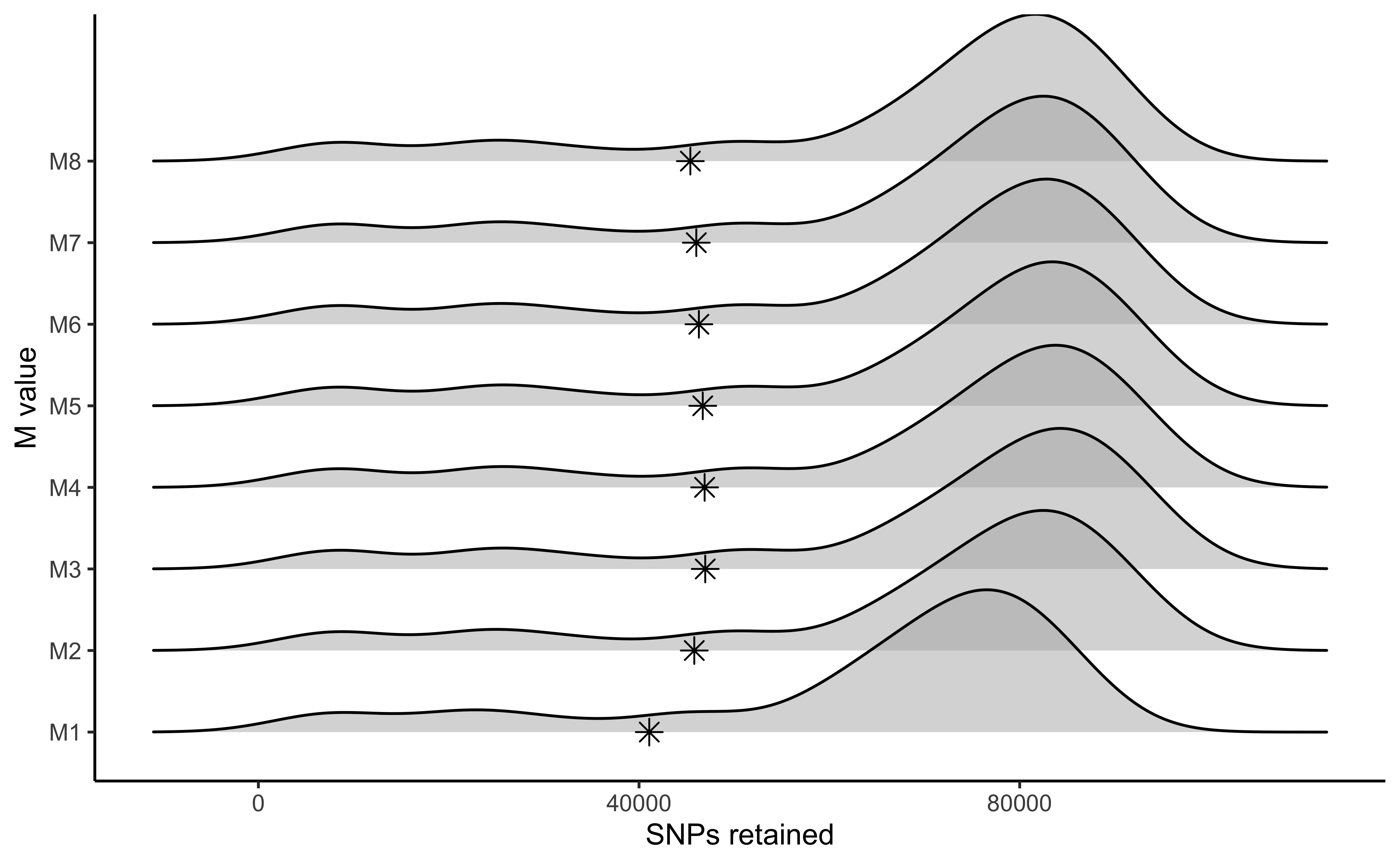


#visualize the effect of varying M on the number of polymorphic loci retained
vis_loci(output = M.out, stacks_param = "M")
#> Visualize how different values of M affect number of polymorphic loci retained.
#> Density plot shows the distribution of the number of loci retained in each sample,
#> while the asterisk denotes the total number of loci retained at an 80% completeness cutoff. The optimal value is denoted by red color.
#> Picking joint bandwidth of 2920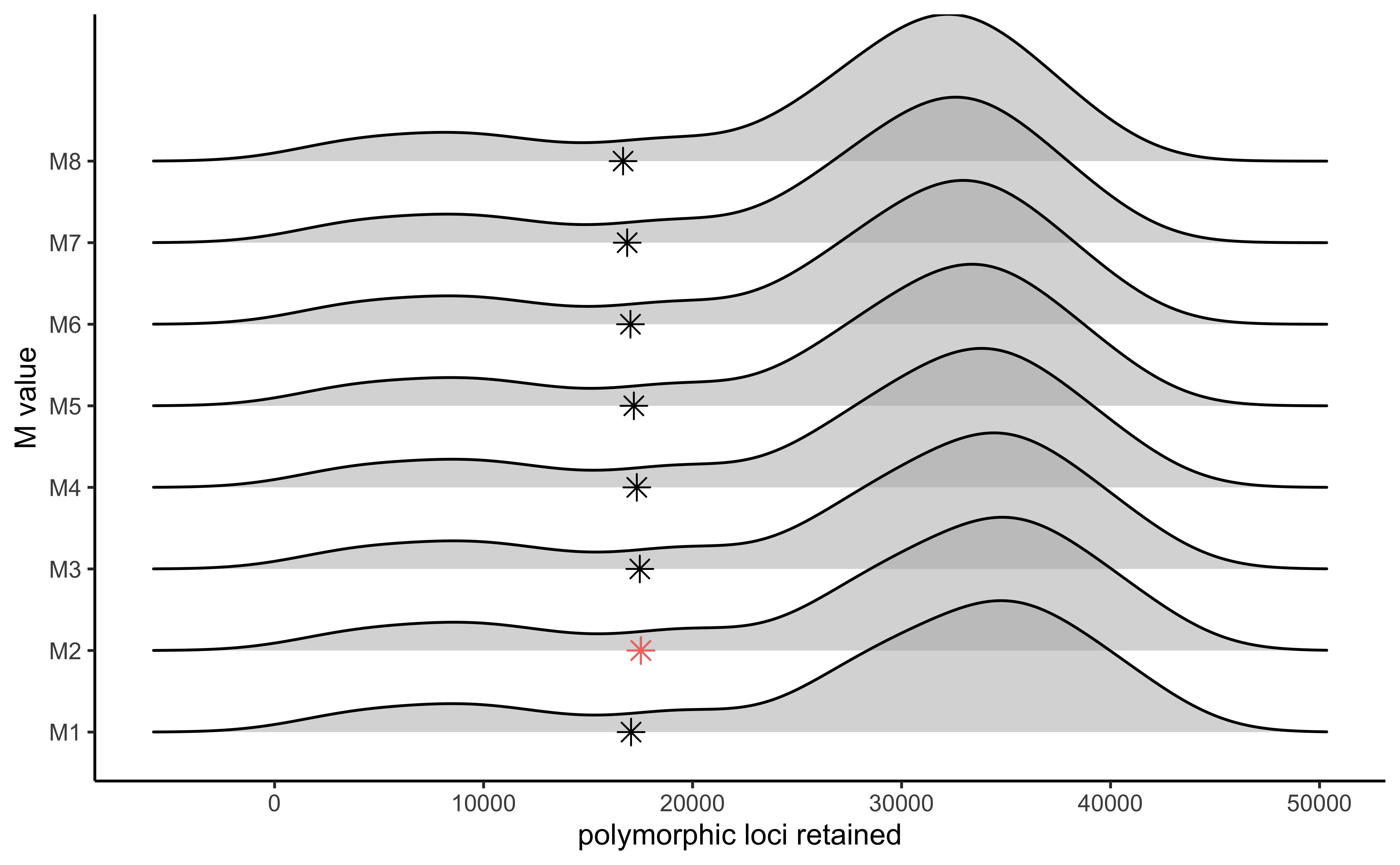

Step 7: Iterate over values of n ranging from M-1, M, M+1, setting m and M to the optimal values (here 3 and 2, respectively).

This code chunk runs the last three Stacks iterations, again re-using the variable $files

# -n — Number of mismatches allowed between sample loci when build the catalog (default 1).
#here, vary 'n' across M-1, M, and M+1 (because my optimized 'M' value = 2, I will iterate over 1, 2, and 3 here), with 'm' and 'M' set to the optimized value based on prior visualizations (here 'm' = 3, and 'M'=2).
for i in {1..3}
do
#create a directory to hold this unique iteration:
mkdir stacks_n$i
#run ustacks with n equal to the current iteration (1-3) for each sample, m = 3, and M=2
id=1
for sample in $files
do
    /home/d669d153/work/stacks-2.41/ustacks -f ${sample}.fq.gz -o stacks_n$i -i $id -m 3 -M 2 -p 15
    let "id+=1"
done
/home/d669d153/work/stacks-2.41/cstacks -n $i -P stacks_n$i -M pipeline_popmap.txt -p 15
/home/d669d153/work/stacks-2.41/sstacks -P stacks_n$i -M pipeline_popmap.txt -p 15
/home/d669d153/work/stacks-2.41/tsv2bam -P stacks_n$i -M pipeline_popmap.txt -t 15
/home/d669d153/work/stacks-2.41/gstacks -P stacks_n$i -M pipeline_popmap.txt -t 15
/home/d669d153/work/stacks-2.41/populations -P stacks_n$i -M pipeline_popmap.txt --vcf -t 15
done

Step 8: Visualize the output of these 3 runs and determine the optimal value for n.

#optimize n
n.out<-optimize_n(nequalsMminus1="/Users/devder/Desktop/hipposideros/n1.vcf",
           nequalsM="/Users/devder/Desktop/hipposideros/n2.vcf",
           nequalsMplus1="/Users/devder/Desktop/hipposideros/n3.vcf")

#visualize the effect of varying n on the number of SNPs retained
vis_snps(output = n.out, stacks_param = "n")
#> Visualize how different values of n affect number of SNPs retained.
#> Density plot shows the distribution of the number of SNPs retained in each sample,
#> while the asterisk denotes the total number of SNPs retained at an 80% completeness cutoff.
#> Picking joint bandwidth of 7420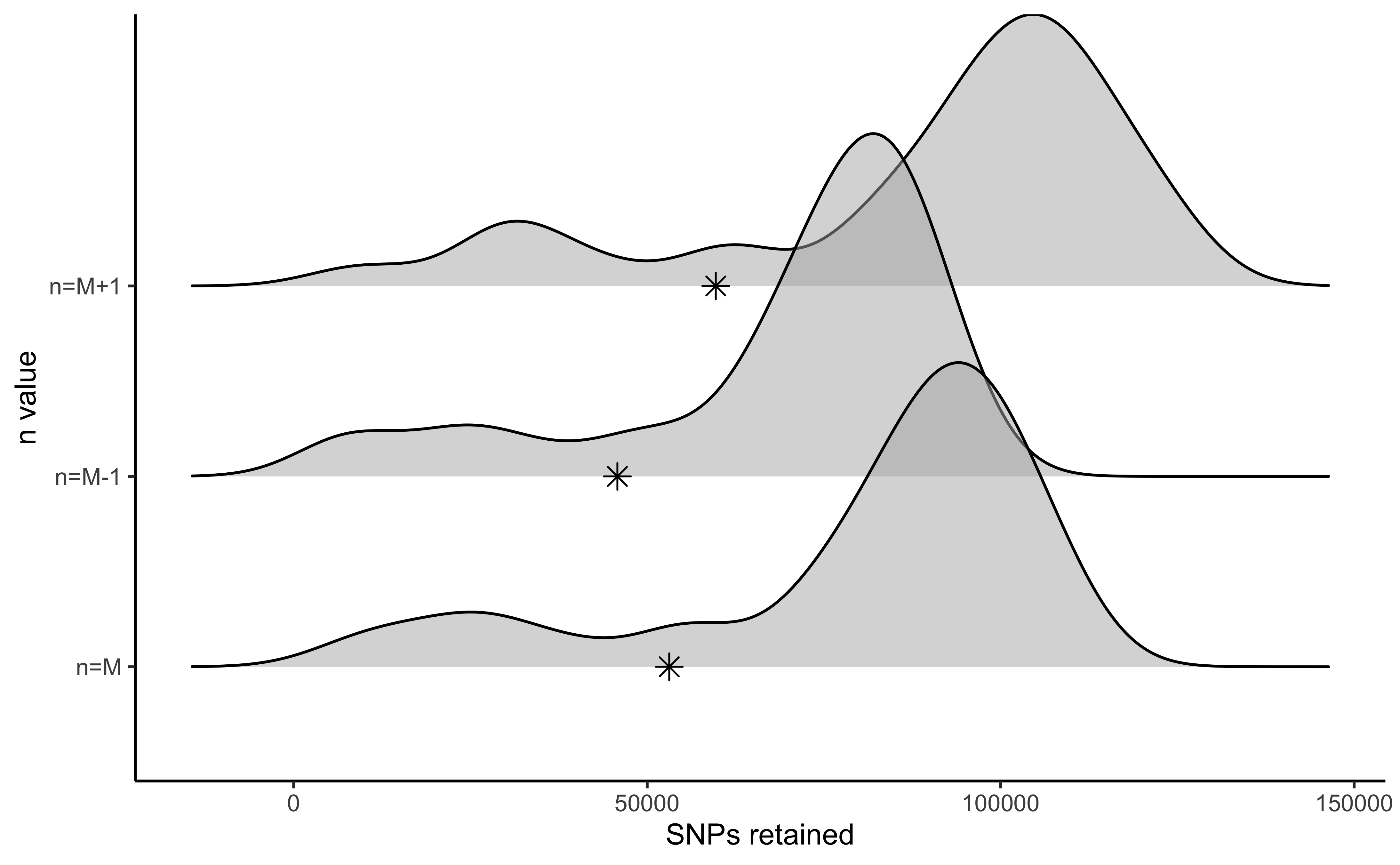


#visualize the effect of varying n on the number of polymorphic loci retained
vis_loci(output = n.out, stacks_param = "n")
#> Visualize how different values of n affect number of polymorphic loci retained.
#> Density plot shows the distribution of the number of loci retained in each sample,
#> while the asterisk denotes the total number of loci retained at an 80% completeness cutoff. The optimal value is denoted by red color.
#> Picking joint bandwidth of 3230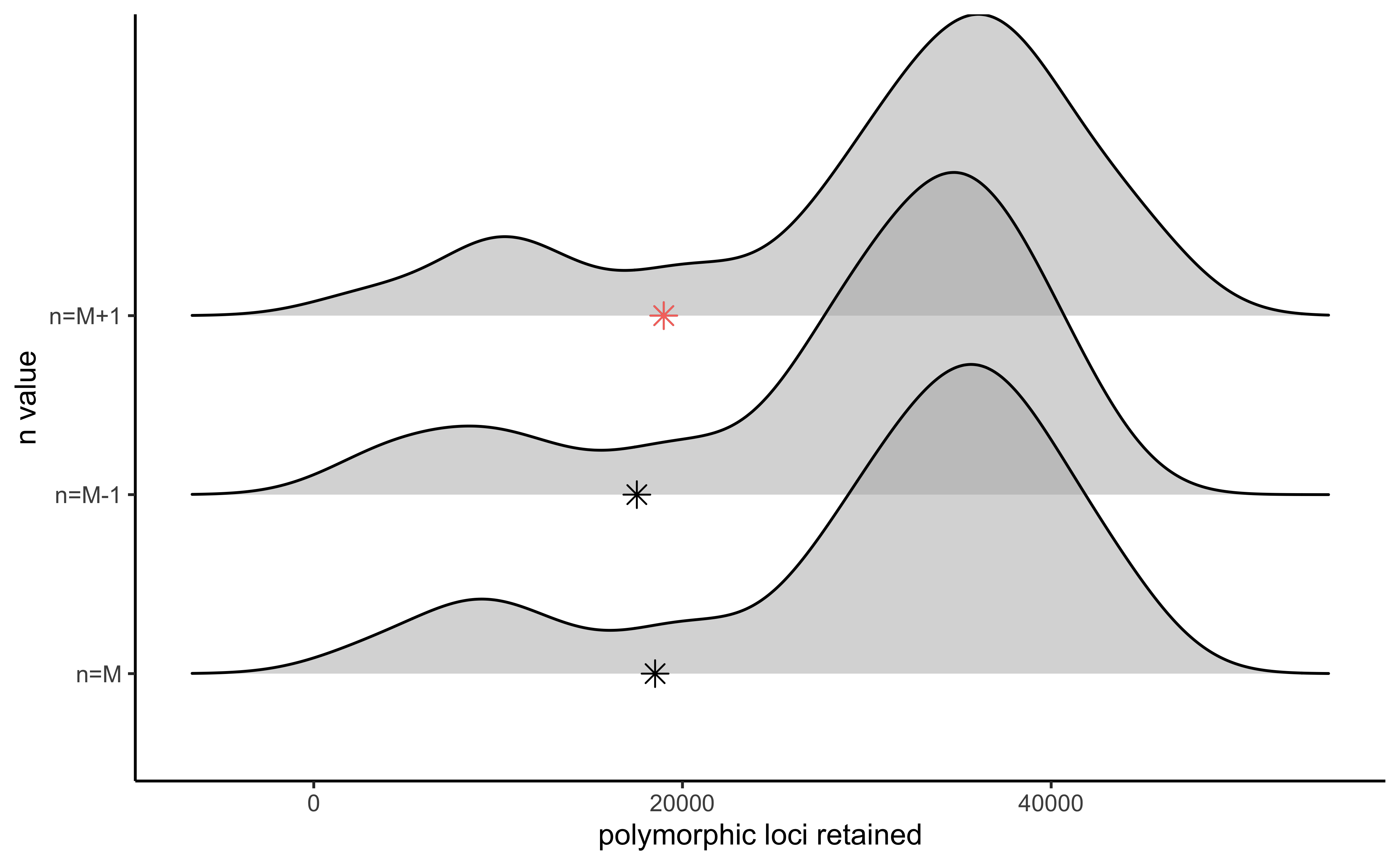

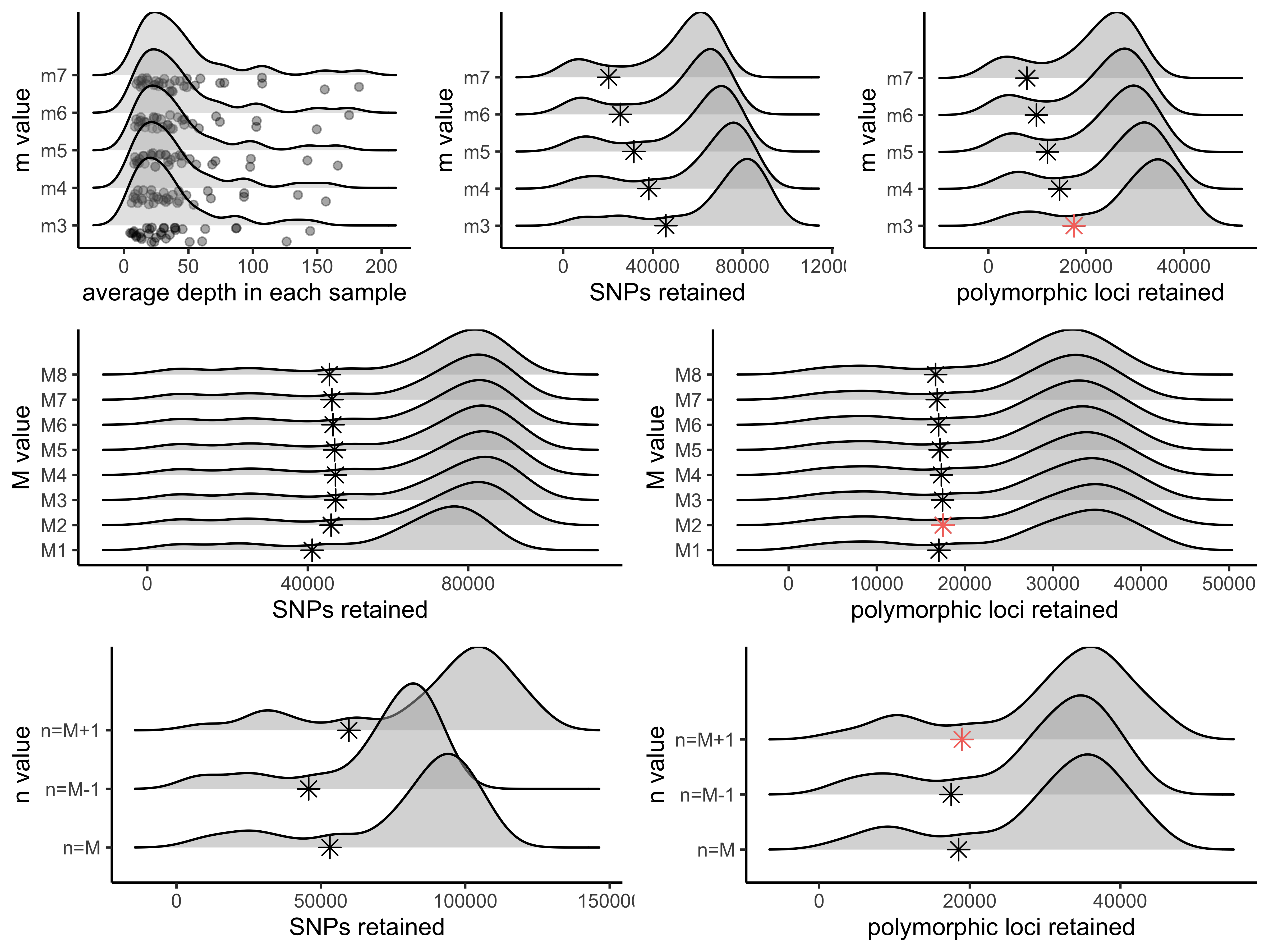
Finally, make a single figure showing the optimization process of all three parameters

gl<-list()
gl[[1]]<-vis_depth(output = m.out)
#> [1] "Visualize how different values of m affect average depth in each sample"
gl[[2]]<-vis_snps(output = m.out, stacks_param = "m")
#> Visualize how different values of m affect number of SNPs retained.
#> Density plot shows the distribution of the number of SNPs retained in each sample,
#> while the asterisk denotes the total number of SNPs retained at an 80% completeness cutoff.
gl[[3]]<-vis_loci(output = m.out, stacks_param = "m")
#> Visualize how different values of m affect number of polymorphic loci retained.
#> Density plot shows the distribution of the number of loci retained in each sample,
#> while the asterisk denotes the total number of loci retained at an 80% completeness cutoff. The optimal value is denoted by red color.
gl[[4]]<-vis_snps(output = M.out, stacks_param = "M")
#> Visualize how different values of M affect number of SNPs retained.
#> Density plot shows the distribution of the number of SNPs retained in each sample,
#> while the asterisk denotes the total number of SNPs retained at an 80% completeness cutoff.
gl[[5]]<-vis_loci(output = M.out, stacks_param = "M")
#> Visualize how different values of M affect number of polymorphic loci retained.
#> Density plot shows the distribution of the number of loci retained in each sample,
#> while the asterisk denotes the total number of loci retained at an 80% completeness cutoff. The optimal value is denoted by red color.
gl[[6]]<-vis_snps(output = n.out, stacks_param = "n")
#> Visualize how different values of n affect number of SNPs retained.
#> Density plot shows the distribution of the number of SNPs retained in each sample,
#> while the asterisk denotes the total number of SNPs retained at an 80% completeness cutoff.
gl[[7]]<-vis_loci(output = n.out, stacks_param = "n")
#> Visualize how different values of n affect number of polymorphic loci retained.
#> Density plot shows the distribution of the number of loci retained in each sample,
#> while the asterisk denotes the total number of loci retained at an 80% completeness cutoff. The optimal value is denoted by red color.

grid.arrange(
  grobs = gl,
  widths = c(1,1,1,1,1,1),
  layout_matrix = rbind(c(1,1,2,2,3,3),
                        c(4,4,4,5,5,5),
                        c(6,6,6,7,7,7))
)
#> Picking joint bandwidth of 9.53
#> Picking joint bandwidth of 7190
#> Picking joint bandwidth of 3420
#> Picking joint bandwidth of 6090
#> Picking joint bandwidth of 2920
#> Picking joint bandwidth of 7420
#> Picking joint bandwidth of 3230

I now have a vcf file containing unfiltered SNPs for all samples, built with the optimal parameters for this dataset, ‘m’ = 3, ‘M’ = 2, and ‘n’=3.

I will now filter this vcf file using the SNPfiltR R package, to generate a set of high quality SNPs for downstream phylogenetic/population genetic analyses.

Optimize denovo STACKS pipeline for Hipposideros bats

This is a real example of using the RADstackshelpR package to facilitate parameter optimization on an empirical dataset. Bash code used to run the STACKS pipeline was executed via submit script on the KU high-performance computing cluster.

Step 1: Demultiplex each sample using ‘process_radtags’.

Step 3: Now that we have run quality control, we have a reasonable set of samples for which to perform parameter optimization for de novo assembly. To begin, iterate over values of ‘m’ ranging from 3-7, while leaving all other parameters at default values.

Note: The vcf file output by Stacks containing only variant site information for each sample will be called ‘populations.snps.vcf’, unless you renamed it yourself by setting the -o flag in populations. This is the vcf file that you want to use for input to RADstackshelpR functions.

Step 4: Visualize the output of these 5 runs and determine the optimal value for m.

Step 5: Iterate over values of M ranging from 1-8, setting m to the optimal value (here 3).

This code follows the bash chunk above, utilizing the same variable $files

Step 6: Visualize the output of these 8 runs and determine the optimal value for M.

Step 7: Iterate over values of n ranging from M-1, M, M+1, setting m and M to the optimal values (here 3 and 2, respectively).

This code chunk runs the last three Stacks iterations, again re-using the variable $files

Step 8: Visualize the output of these 3 runs and determine the optimal value for n.

Finally, make a single figure showing the optimization process of all three parameters

I now have a vcf file containing unfiltered SNPs for all samples, built with the optimal parameters for this dataset, ‘m’ = 3, ‘M’ = 2, and ‘n’=3.

I will now filter this vcf file using the SNPfiltR R package, to generate a set of high quality SNPs for downstream phylogenetic/population genetic analyses.